Introduction

I’m sure every data scientist starts their data science journey by pumping those accuracy scores, trying to squeeze out an extra 0.5% to move their 99% accurate model to 99.5% while also trying to maintain a healthy balance of preventing overfitting, but all that mattered then, especially for those Kaggle, Zindi hackathons then was accuracy. But as we all progress up the data science ladder, we begin to learn about precision, recall, F1-score and how they are better means of evaluating our model performance. So how do you know when to use which (accuracy, precision, recall and f1-score)? In this article, I’ll be taking you through that giving you a real industry perspective also. Let’s get right into it.

Getting Started

So before we proceed to understand what actually is accuracy, precision, recall and f1-score are, let’s, first of all, create a sample dataset and simple model that we will use to explain these concepts.

import numpy as np
from sklearn.datasets import make_classification

X, Y = make_classification(n_samples = 500,
                          n_features = 10,
                          n_informative = 5,
                          n_redundant = 5,
                          n_classes = 2,
                          weights = [0.75, 0.25],
                          random_state = 27)

We are trying to create a simulated classification dataset that we’ll be using with 500 rows, and 10 columns out of which only 5 are informative and 5 are noise. The data has 2 classes 0 and 1 with 400 zeros and 100 ones. Next, we want to confirm that the dataset we created is just as expected and view the first 5 rows of X and the first 100 of Y

X.shape

(500, 10)

Y.shape

(500,)

X[:5, :]

array([[-0.32718827, 1.24378523, -1.63117202, 1.70196308, 3.22607374, 0.12536251, -1.32531688, -1.5178169 , 0.0391831 , 5.37803965], [-0.18882151, 3.24450273, -0.04684192, 0.42667327, 0.95977818, -1.41401465, 0.6218516 , -2.76514217, -1.35078041, 1.62561421], [-1.32438294, -2.56364318, -3.10395577, -0.71218974, 2.06383318, 2.2750899 , -0.41726115, 3.39746801, 0.48384514, 0.00984739], [ 2.72758704, 0.01696436, 0.8414895 , -0.42127927, 2.0270105 , 3.09904819, -0.80473595, 2.5118864 , -2.07646986, -0.56676343], [ 2.83704055, -1.64725719, 1.04781064, 1.69459622, 1.951591 , 1.24457155, -0.03491821, 2.14001566, 0.51324065, 0.93051073]])

Y[:100]

array([1, 1, 0, 1, 1, 0, 0, 0, 0, 0, 0, 0, 0, 1, 0, 0, 0, 0, 0, 0, 0, 1, 1, 0, 0, 0, 0, 0, 0, 0, 0, 1, 1, 0, 0, 0, 0, 1, 0, 0, 1, 1, 0, 0, 0, 0, 0, 1, 0, 1, 1, 0, 0, 0, 0, 0, 0, 1, 0, 1, 0, 0, 0, 1, 0, 0, 1, 0, 0, 0, 0, 0, 0, 0, 0, 0, 1, 0, 0, 0, 0, 0, 0, 0, 0, 1, 0, 0, 0, 0, 1, 0, 0, 1, 0, 0, 1, 0, 0, 0])

Next, let’s split our dataset to train and test set

from sklearn.model_selection import train_test_split

X_train, X_test, Y_train, Y_test = train_test_split(
                                X,Y, test_size=0.2, random_state=27)

We split our dataset to keep 20% (100 rows) as test_size and use others to train. Next, let’s ascertain the size of our splits

X_train.shape

(400, 10)

Y_train.shape

(400,)

X_test.shape

(100, 10)

Y_test.shape

(100,)

Next, let’s create a simple Logistic Regression model to train our dataset.

from sklearn.linear_model import LogisticRegression

logit = LogisticRegression(random_state=27)
model = logit.fit(X_train, Y_train)
Y_hat = model.predict(X_test)
Y_proba = model.predict_proba(X_test) 
Y_proba.shape

(100,2)

Next, we’ll be importing the metrics we’ll be using to evaluate our model

from sklearn.metrics import accuracy_score

print(f"Training accuracy: {model.score(X_train, Y_train)}")
print(f"Test accuracy: {model.score(X_test, Y_test)}")

Training accuracy: 0.8175

Test accuracy: 0.75

Also before we dive into the theory behind the topics, I’ll write a helper function that will help us tinker with our prediction, I’ll explain briefly what it does after

def set_threshold(Y_proba, threshold):
    Y_hat = []
    for x in Y_proba[:, 1]:
        if x > threshold: Y_hat.append(1)
        else: Y_hat.append(0)
    return Y_hat

This helper function basically helps us set the boundary for our decisions. Our logistic regression gives a probability of our inputs being the 0 or 1, there are two columns when we use model.predict_proba (which we’ll be using for this analysis) instead of model.predict. Logistic regression thus uses a default threshold of 0.5, which means if for the predictions Y_proba[:,0] (all rows of probability predictions of 0), if the model is more than 50% sure (i.e value is greater than 0.5), then return 0 for that row, else it is 1. The same thing for the second column representing 1 (don’t forget, the sum of both rows equals 1), so we’ll be selecting just the second row, if the value is greater than our threshold (in case we want greater confidence, let’s say 80% in our predictions or lower confidence), it should return 1, if not, it’s automatically a 0.

Under the hood

So what exactly is accuracy, precision or recall? To understand that, we’ll need to first understand what a confusion matrix is.

Confusion matrix

So a confusion matrix is a two-by-two matrix where the rows represent the actual values while the columns represent the predicted values

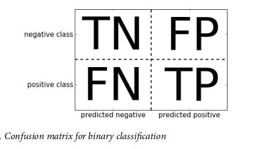
For the sake of this analysis, 1 will be our positive value while 0 will be the negative value. The four constituents of a confusion matrix as shown above are TN, FN, FP and TP

• True Negatives (TN): This represents the actual negative values (0 in our case) that the model predicted as negative.
• False Negative (FN): This represents values that are actually positive but or model predicted as negative (actually 1 but predicted as 0).
• False Positives (FP): This represents values that are actually negative but our model predicted as positive (actually 0 but predicted as 1).
• True Positive (TP): This represents values that are true and our model also predicted as true (1 predicted as 1 also).

This means the first row represents all values that are actually negative (0), while the second row represents values that are actually positive (1). The first column thus also represents all the values our model predicted as negative (0) while the second column represents the values our model predicted as positive (1). Before we proceed any further, let us create the confusion matrix for the initial prediction.

from sklearn.metrics import confusion_matrix

confusion_matrix(Y_test, Y_hat)

array([[65,  3],
       [22, 10]])

[Note that the values inside confusion_matrix function are positional, it expects the base truth (Y_test) as the first argument and the predictions (Y_hat) as the second, anything apart from this can mess up your analysis].

Thus, we can assign the values as follows TN (65), FN (22), FP (3) and TP (10). Now that we understand what a confusion matrix is, we can move on to others.

Accuracy

Accuracy is therefore the sum of actual correct predictions (TP and TN) by our model, divided by total test data size, simply,

 Accuracy = (TN + TP)/(TN+ FN + FP + TP).

This gives a simplistic overview of how correct our model is, nothing more than that. This means the accuracy of our model is

Accuracy = (65 +10)/(65 + 22 + 3 + 10)
=   75/100
= 0.75

Precision

Precision however tells us of how many of the values our model predicted as positive are actually positive.

Precision = TP/(TP + FP)

This means the precision for our model is

Precision = 10/(10+3)
    = 10/13
    = 0.7692

Precision is used when there is a great cost for FPs, I’ll explain this very soon

Recall

Recall tells us how many of the actual positive value is captured as positive by our model. This calculated using

Recall = TP/(FN + TP)

This means the recall for our model is

Recall = 10/(22+10)
            = 10/32
            = 0.3125

Recall on the other hand is used when there is a great cost for every FN. This I’ll also explain soon. These values can be gotten simply in sklearn using the classification_report method from metrics.

from sklearn.metrics import classification_report

print(classification_report(Y_test, Y_hat))

                   precision    recall  f1-score   support

                    0      0.75      0.96      0.84        68
                    1       0.77      0.31      0.44        32

     accuracy                                 0.75       100
     macro avg       0.76      0.63      0.64       100
 weighted avg       0.75      0.75      0.71       100

[Note that the values inside classification_report function are positional, it expects the base truth (Y_test) as the first argument and the predictions (Y_hat) as the second, anything apart from this can mess up your analysis]

This gives the precision, recall, f1 score (to be explained also) of each class and weighted accuracy.

When to use which

So if you’re observant, you’ll notice two things, first, the precision of 0 is relatively good (0.75) and the recall is even much higher (0.96) even though the accuracy is 0.75. This happened because our dataset is unbalanced (this means the two classes are not of the same number or weight, we have 68 values that are actually zeros and 32 values that are ones). The implication of this is that if we set our model to return the highest class (0) for every prediction, our model will have an accuracy of 0.68 (since we will get all 0s and miss all 1s). This point to the fact that accuracy is not a reliable metric to evaluate a model in cases of unbalanced dataset (e.g cancer detection, where out of 100,000 thousand people screened just 10 people might actually have cancer).

The other thing to note is that the recall and precision of 1 are like inversely proportional. This is because if we want high precision, we need our model to be very confident that the prediction it is making is actually positive, thus any value that is actually positive but our model is not so confident about i.e didn’t meet our threshold will be set as positive. This means the actually positive values will be the majority of values that our model will predict as positive. This also then implies that, the cost of this high precision will a lot of actually positive values but which our model is not confident about will be classified as negative, therefore we will have a lot of false negatives. This implies that the values our model will predict as positive will actually be a very small fraction of actually positive values, thus low recall. The inverse will give a high recall and low precision.

Lets's go through this using business case studies.

Business case studies

Here I’ll be showing two different case studies;

• Fraud detection
• Drug discovery

using different thresholds so that we can have a very high recall for one and very high precision for the other. A little introduction to our case studies to understand their business needs.

Fraud detection

X is a new fintech startup that is trying to compete in the neobank space with Kuda, Carbon, Renmoney et al in Nigeria and Africa. But there is a problem, fraud is rampant in the space. So they are employing you as a data scientist to build a machine learning model to detect whether a transaction is fraudulent or not. As the data scientist, you have built a fairly accurate model using Logistic Regression but you understand that accuracy won’t tell you the full picture, so you need something to give you more insight about your model and whether to increase your threshold for what you classify as fraud or not, so let’s break this down using the confusion matrix for what the result for each prediction will be on the business.

• True Positive: These are transactions that are actually frauds and your model also predicted as frauds. You want to increase this to capture all fraudulent transactions as actual frauds.
• True Negative: These are transactions that are not frauds (i.e normal transactions between your customers) and your model predicted correctly too.
• False Positive: These are normal transactions between your users but your model flagged as fraud. By flagging them, the users will have to contact your boss that they are the ones performing the transactions and are not committing any fraud. This may cause your customers inconvenience and make your company’s service offering not as sleek as they need it to be. If it consistently flags people from a particular region or demography, your company may receive public out-lash that it is biased and people from that region may boycott your product and others who want to stand in solidarity. You want to reduce this to as low as possible.
• False Negatives: These are transactions that are actually frauds but your model predicted that they are not. As a data scientist in this company, you don’t even want to see this at all because it threatens both your company and your job. If you model often flag transactions that are frauds as not fraud, your company will have to pay that money back to the client or pay several damages if many people sue, so the company may use all the runway money to pay damages and you people will pack up or if not, your CEO may think maybe you’re conniving with the fraudsters to give them easy passage and sue you or even think you’re probably not good enough in your job and end up sacking you to employ another person. (These are just hypothetical scenarios).

So you understand that while you want to reduce both the FP and FNs, your customers may still understand FP scenarios a bit, they won’t tolerate FN at all. This means there is a greater cost associated with FN than FP. Thus, the goal is to have the best recall as high as possible while maintaining relatively good precision and accuracy

Drug discovery.

Y is a new tech-enabled pharmaceutical company that is trying to bring a new drug to market. Drug discovery is a very expensive and time-consuming process with a new drug taking an average of about 10 years before getting to the market and requiring an estimated $10 billion. Because your company is tech-focused, they employed you as a data scientist to build a machine learning model on top of the High Virtual Through Put Screening (HTVS) to determine whether a new compound will be a potential drug but there is a potential cost of $100k to evaluate and carry out necessary tests to check whether the compound will actually be useful. So as a data scientist, you have also built a simple model using logistic regression and want to evaluate the model better beyond just accuracy to using confusion matrix, precision and recall. So let’s break down using the confusion matrix what each prediction means and the business impact:

• True Positive: These are actual compounds that have a therapeutic activity that your model predicted as positive compounds, you want to optimise this as much as possible.
• True Negative: These are compounds that actually have no therapeutic activity and your model predicted correctly as negative compounds not to take note of. You also want to maintain this.
• False Negative: These are compounds that actually have therapeutic values but our model predicted as negative (that they have no therapeutic value). You want to reduce this as much as possible because those are potential compounds that may be the solution to some of the biggest health challenges globally and may have the highest ROI (return on investment).
• False Positive: These are compounds that don’t actually have any therapeutic value or are even toxic but our model predicted them as positive (i.e they have therapeutic importance). You don’t even want to see these at all because, for every one of them, that is $100k going down the drain, this means 10 FPs is $ 1 million all for nothing, that’s a lot of money your company is looking for you to save for them. (These are just hypothetical scenarios).

So based on this, while we want to reduce both FP and FN, we can see that there is a greater cost to FP compared to FN, thus, our priority is having the best precision possible while maintaining relatively good recall and the accuracy too.

Original model

So here’s a copy of the result of our initial model (with the threshold set to 0.5), its confusion matrix, accuracy, precision and recall.

Y_50 = set_threshold(Y_proba, threshold=0.5)
print("Confusion matrix with thresh = 0.5 \n",
      confusion_matrix(Y_test, Y_hat))

Confusion matrix with thresh = 0.5 
 [[65  3]
 [22 10]]

print(classification_report(Y_test,Y_50))

                       precision    recall  f1-score   support

                   0      0.75      0.96      0.84        68
                   1       0.77      0.31      0.44        32

   accuracy                                  0.75       100
    macro avg       0.76      0.63      0.64       100
weighted avg       0.75      0.75      0.71       100

• Fraud detection: For our fraud detection scenario, the model has an accuracy of 0.75, a precision of 0.77 and a recall of 0.31. The accuracy and precision are fairly good but the recall is bad. Remember, recall means the number of the actual positive value that our model captured as true and we need to optimise our fraud detection model to have the best recall (low FNs). The implication of that recall means that our model is only flagging 10 out of 32 fraudulent transactions as fraudulent while fraudsters are having a swell time with the remaining 22 transactions. This implies that with our 77% precision, this is a really bad model.

• Drug discovery: For our drug discovery model, a precision of 77% means out of 13 compounds that our model predicted as potential drugs, 10 are actual potential drugs while just 3 are wrong, while there is a huge cost on the 3 errors this is still a relatively good model, the cost is not that much and given that we were able to identify 10 potential drugs out 100 that we were given. The poor recall shows that we are missing out on a lot of potential compounds that may be potential drugs, but we are at least not wasting money chasing compounds that actually are not. In summary, this is a relatively good model for our drug discovery.

Lower threshold

Next, we’ll set a lower threshold/ confidence limit of 0.3 for our model, this means probability predictions of 1s greater than 0.3 will be classified as 1 or otherwise as 0.

Y_30 = set_threshold(Y_proba, threshold=0.3)
print("Confusion matrix with thresh = 0.3 \n",
      confusion_matrix(Y_test, Y_30,))

Confusion matrix with thresh = 0.3 
 [[59  9]
 [ 8 24]]

print(classification_report(Y_test, Y_30))

                        precision    recall  f1-score   support

                    0       0.88      0.87      0.87        68
                     1       0.73      0.75      0.74        32

        accuracy                                 0.83       100
      macro avg       0.80      0.81      0.81       100
weighted avg       0.83      0.83      0.83       100

• Fraud detection: This model has much higher accuracy and recall compared to the last model but slightly lower precision. Analysis of this model shows that it accurately predicts 24 out of 32 fraudulent transactions as actually fraudulent. This is a lot better model than the previous model. Even though the false negatives are a bit still high (8), it is a lot better than the previous (22). The slightly lower precision and confusion matrix showed we have more false positives i.e more customers whose normal transactions we are flagged as fraudulent and have to be put through the stress of proving themselves compared to the previous model (with 3) but in all, this is a lot better model for us.

• Drug discovery: For our drug discovery model, the higher recall means this is a great model, we have been able to identify more potential drugs (24) compared to the former model (10). That is definitely great business. The slight drop in precision means compared to 3 false positives that the previous model gave, this model gave 9, the financial implication of that is the company is wasting an additional $600K more than the $300k lost to false predictions of the previous model totally $900K. That’s definitely not so great business. This means that even though this improved model gave us more compounds, our losses tripled. Depending on who you ask and how you look at it, it seems the previous model is better than this.

Higher threshold

For this final model, we want to set the threshold/ confidence limit of our model to be very high (0.8).

Y_80 = set_threshold(Y_proba, threshold=0.8)
print("Confusion matrix with thresh = 0.8 \n",
      confusion_matrix(Y_test, Y_80,))

Confusion matrix with thresh = 0.8 
 [[68  0]
 [29  3]]

print(classification_report(Y_test, Y_80))

                         precision    recall  f1-score   support

                     0      0.70      1.00      0.82        68
                     1       1.00      0.09      0.17        32

         accuracy                                 0.71       100
     macro avg       0.85      0.55      0.50       100
 weighted avg       0.80      0.71      0.62       100

• Fraud detection: While the accuracy of this model (0.71) is not so far from the first model (0.75), it seems this is the worst model in the fraud detection case study, even though the precision is very high at 1.00 meaning we falsely classified no transaction as fraud that wasn’t actually a fraud (all transactions classified as fraudulent are fraudulent), the cost is that we only classified 3 values as fraud while falsely classifying 29 transactions that are actually fraudulent as not fraudulent. This is a very bad model, a very bad one.

• Drug discovery: This precision of 1 of this model means that out of 3 values that we predicted as potential drugs, all the 3 are potential drugs. This is a really great model because we are not going to be wasting any money on any compound only to discover that is not a potential drug. For a small company with limited funds, this is a great model even though they’ve missed out on a lot of other potential drugs. Depending on the size of the company and if they have any money to spare, if they are a small company with no money to spare, this is the best model for them. If they have some cash that they can burn, then the first model might be the best for them or if they are a large established company with all the money to burn just to get the best ROI, then the second model is for them.

F1 score

So I have explained precision and recall and how they are both inversely proportional. What about times when we want to keep an eye on both our precision and recall using a single value? F1 Score provides us with a value to keep an eye on both precision and recall simultaneously, it represents the harmonic mean of precision and recall and is given by

F1 score = 2 * (precision * recall)/ (precision + recall)

The higher the F1 score, the relatively high values for both the precision and recall, if not, then one of the two values is really low. This shows in our dataset as the third model has an F1 score of 0.17 as the recall was 0.09 even though the accuracy was 0.71. The first model also had an F1 score of 0.44 because the recall was 0.31 even though the accuracy was 0.75, the second model which had relatively high precision and recall also had a high f1 score of 0.74 and even higher accuracy of 0.83.

In this article, I explained comprehensively precision, recall, accuracy and f1 score while considering business case studies and the considerations that go on behind the scene in selecting the best evaluation metric. If you found this article useful, please share it with someone who might also benefit from it. You can also share positive feedback in the comments or follow me on Twitter @madeofajala. Till next time, see ya...